Sensor Fusion

Reference vedio
1. Theory description
- overcomve limitations of individual sensors
- estimate quantities that are not directly measured
Example: Aircraft Attitude Estimation (using Accelerometer and Gyroscope)
- describe the orientation by roll ($\phi$), pitch ($\theta$) and yaw ($\psi$) angles w.r.t a fixed coordinate system
- the measurement of gyroscopes (p, q, r) are not equal to ($\dot{\phi}$, $\dot{\theta}$, $\dot{\psi}$)
- measure accelerations of all axis: $a = [a_{x}, a_{y}, a_{z}]~ (m/s^{2})$
- Accelerameter model
-
If the accelerometer is at rest, we can get $\phi$ and $\theta$ from:
- $a_{x} = g * \sin(\theta)$
- $a_{y} = -g * \sin(\phi) * \cos(\theta)$
- $a_{z} = -g * \cos(\phi) * \cos(\theta)$
-
and get:
- $\hat{\phi}_{acc} = \tan^{-1}(\frac{a_y}{a_z})$
- $\hat{\theta}_{acc} = \sin^{-1}(\frac{a_x}{g})$
-
Practical considerations
- only close to true at rest
- noise term: HF noise and need low-pass filter to measurements
- Time-varying bias: how to estimate? initial calibration?
- Measures angular rate of rotation around each axis: $\omega_b = [p, q, r]~ (rad/s)$
- Gyroscope model
-
Need to transfrom body rates to Eulaer rates:
- $\dot{\phi} = p + \tan(\theta) * (q * \sin(\phi) + r * \cos(\phi))$
- $\dot{\theta} = q * \cos(\phi) - r * \sin(\phi)$
- $\dot{\psi} = \frac{q * \sin(\phi) + r * \cos(\phi)}{\cos(\theta)}$
-
Practical considerations
- fixed sampling time T
- we need to know $\phi$ and $\theta$ to get $\dot{\phi}$ and $\dot{\theta}$
- Can’t simply get them by integrating $\dot{\phi}$ and $\dot{\theta}$ from accelerometer measurements, due to time-varying bias, which leads to gyro drift
- need low-pass filter and optional very low cutoff high-pass filter
- Conclusions
- Accelerometer is good at estimating attitude when the object is at rest
- Gyroscope is good at estimating attitude over short periods of time
- Need to combine the two to get a good estimate of attitude
2. Complementary Filter

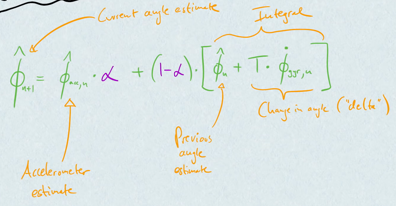
$\hat\phi_{n+1} = \hat\phi_{acc,n} * \alpha + (1 - \alpha) * [ \hat\phi_{n} + T * \hat\phi_{gyro,n} ]$
same for $\hat{\theta}$
-
$\alpha$ is a constant between 0 and 1
-
typically $\alpha$ is close to 0 (accelerometer is just to compensate for gyro drift, but usually gyros provide a better estimate)
-
Pratical considerations
- need to know $\phi$ and $\theta$ to get $\dot{\phi}$ and $\dot{\theta}$
- may need to low-pass filter final extimates
- computationally expensive operations: $\sin(), \cos(), \tan()$
- better integration method?
- Initialization
- how to choose $\alpha$?
- how much do we filter measurements?
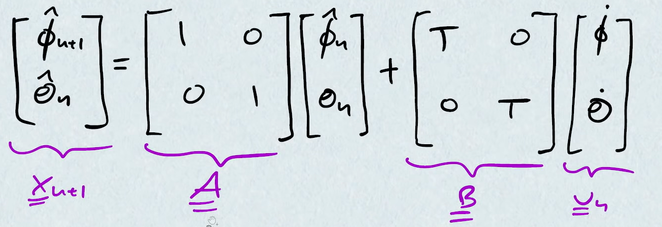
- $\hat x_{n+1} = A * \hat x_{n} + B * u_{n}$
- $\hat{x}$ is state vector
- $A$ is state transition matrix
- $B$ is control input matrix
- $u$ is input vector

and it becomes:

3. Extended Kalman Filter (EKF)
non-linear version of the classical Kalman filter
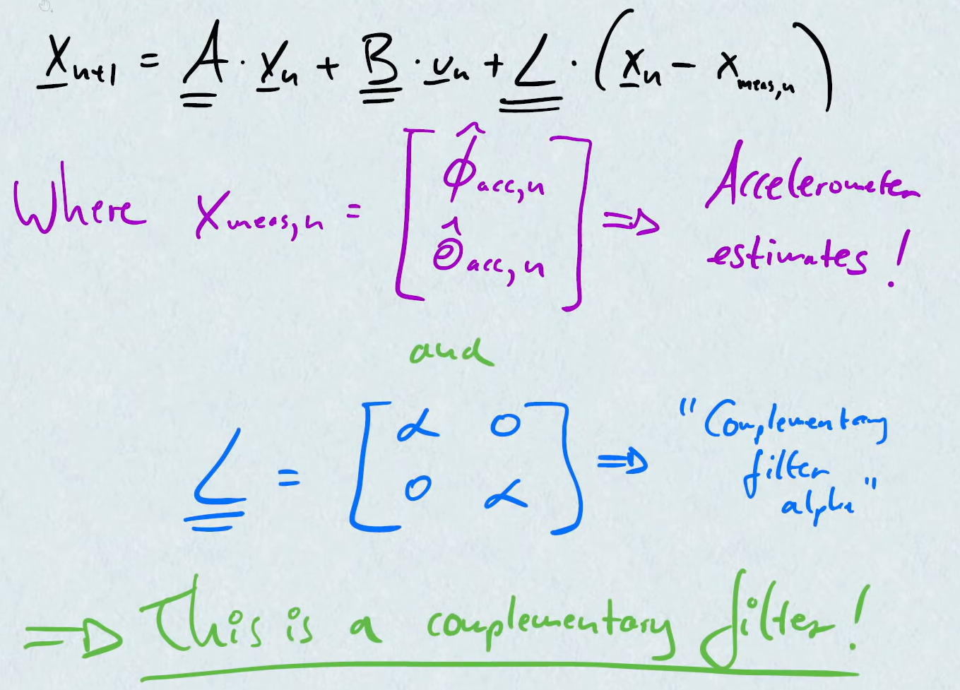
Kalman filter, just like complementary filter, but will optimally choose $\alpha$ for us
- Overviews
- Optinal method of chooseing $\alpha$
- Doesn’t have to be scalar, thus can be used for more complex systems and system sizes
Matrix form of classical observer, K is the Kalman gain and is chosen at every time step:

- estimation error is defined by: $\tilde x = x - \hat x$ (true - eseimate)
- error covariance is defined by: $P = E[\tilde x * \tilde x^T]$
Basic idea: The Kalman filter choose the Kalman gain K, such that the error covariance matrix P is minimized
-
Problems
-
Algorithm
Example: Aircraft Attitude Estimation (using Accelerometer and Gyroscope)


